
Almost Gate: Categorization by Neural Operations
Ten Thousand Neural Inputs Categorize the Diverse Universe by Ignoring Small Differences

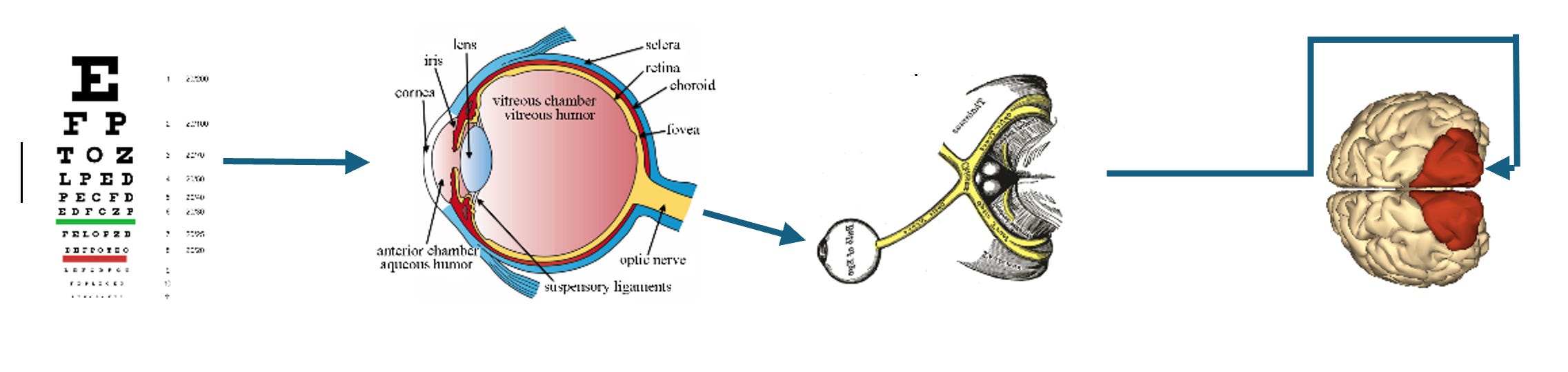
The diagram traces the route of visual information: from raw input at the foveal cones, through preprocessing, into the optic nerve, and onward to the occipital V1 cluster.
This post examines neural operations along that pathway that can be described as Almost Gates. By treating near‑matching inputs as equivalent, Almost Gates suppress trivial differences and allow categorization by inherent properties.
Neural Threshold
The neural threshold is the level of electrical potential a neuron must reach to fire.
The neuron operates as an all‑or‑none signal generator: once the threshold is crossed, the neuron transmits its message to connected neurons.
A neuron’s resting potential is about –70 mV (millivolts).
The firing threshold lies roughly 15 mV above this resting state.
Incoming signals at the dendrites can be ~100 mV, but each synapse passes only a fraction of that strength across the gap.
Synaptic efficiency is not fixed; it changes with experience and learning, altering how signals contribute to reaching threshold.
In a prior post, (Neurons: Engine of Signal Flow) I displayed a cell body with five dendritic branches. In practice, a single neuron may receive input from thousands—sometimes up to ten thousand—dendrites converging on its synaptic gaps
I also introduced the idea of the Almost Gate (Almost Gate by examples) where near matches are treated as identical, and later explored its broader consequences (Layers of Neurons Yield Brain Maps). These links provide background for readers who want the full arc, but the present discussion can be followed without them,
Neural Math Made Simple
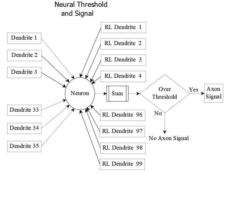
At its core, a neuron’s computation is straightforward: add up the incoming signals, compare the sum to the threshold, and fire if the threshold is achieved or exceeded.
This section presents that process in clear terms — just summation, comparison, and on/off signaling. No advanced math is required, but the equations reveal how neurons transform raw inputs into categorical recognition.
To make the idea concrete, we’ll look at the receiving layer that learns to recognize the English capital letters. Each neuron in that layer aggregates its inputs, and the neuron with the highest potential signals which letter is present.
AI researchers describe this kind of process as unsupervised learning: categories emerge without explicit instruction. It is learning in the strict sense — not teaching, but the brain’s own act of pattern recognition.
Resolving Power and Neural Allocation
To begin constructing the neuron’s input summation, we first assign values to the visual sensors and their receiving layer.
In the occipital lobe, the primary visual cortex (V1) processes input from the fovea with extraordinary density. For the visual space subtended by a single character—roughly one-third of a degree—V1 recruits between 3 and 7 million neurons. To ground the summation, we’ll model the receiving layer as 3 million neurons, a conservative choice within that range.
At the eye’s resolving limit, this stimulus corresponds to approximately 3,000 input elements (pixels), each feeding into the V1 population. This disproportion—thousands of input elements driving millions of cortical neurons—reflects the brain’s strategy for amplifying resolving power through dense neural allocation.
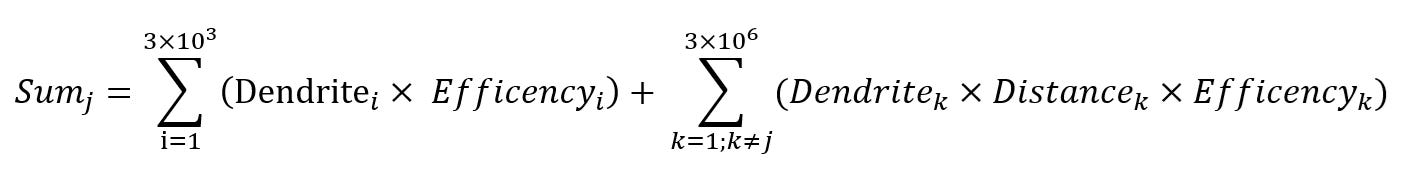
Sumj represents the total input received by neuron j, one of the 3 million neurons in the receiving layer.
The first summation captures direct sensory input: each of the ~3,000 visual units projects signals to neuron j as well as to the other neurons in the layer. These signals arrive at dendrites with varying transmission efficiencies, reflecting the synaptic strength of each connection.
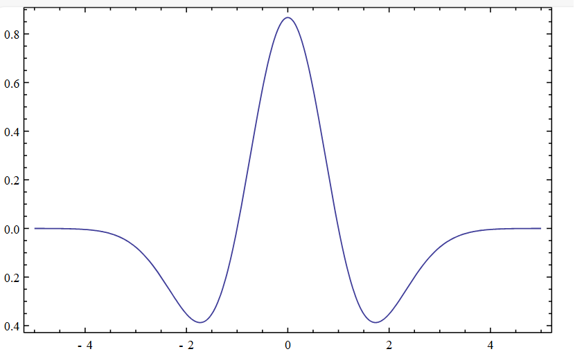
The second summation reflects lateral interactions within the receiving layer. Each neuron is linked to every other neuron via excitatory or inhibitory signals, modulated by their spatial separation. This relationship is governed by the Mexican Hat function—a distance-dependent kernel that assigns positive weights to nearby neurons, negative weights to those slightly farther away, and negligible influence beyond that.
In effect, neurons close to a firing neighbor receive a boost to their input sum; those at intermediate distances are suppressed; and those beyond the kernel’s reach remain unaffected.
Summation with Values
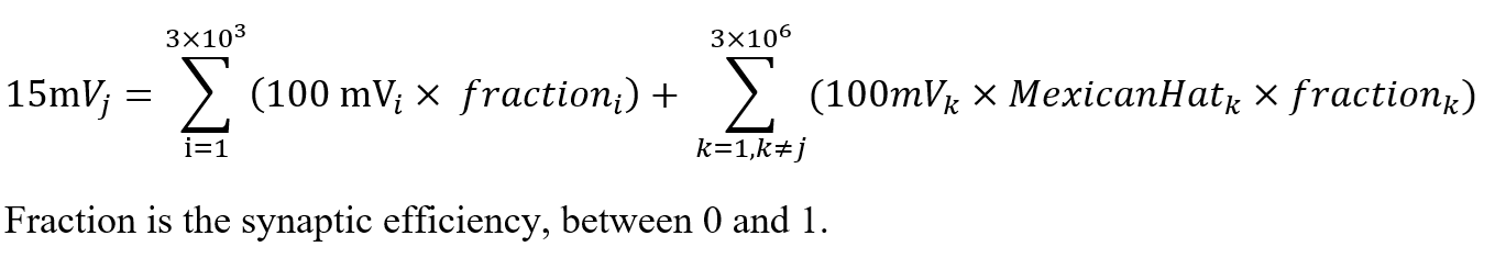
Here, the neural summation becomes more concrete. The total input to neuron , Sumj, is compared against a threshold of 15 mV. If this threshold is met or exceeded, neuron fires—sending a 100 mV signal down its axon to downstream targets.
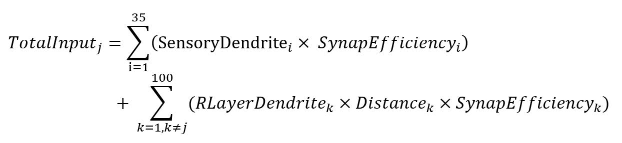
The first summation captures direct sensory input: each of the ~3,000 visual units contributes a signal scaled by its synaptic efficiency—a fraction between 0 and 1 that reflects transmission strength across the synaptic gap.
The second summation accounts for lateral input from other neurons in the receiving layer. Each signal is weighted by the Mexican Hat function, which modulates influence based on distance: nearby neurons are excitatory, those slightly farther are inhibitory, and distant ones exert negligible effect. This spatial weighting is then scaled by each connection’s synaptic efficiency.
Concrete Example
To make the summation more tangible, we shift from the full biological scale to a simplified model. Instead of 3,000 sensory inputs and 3 million receiving neurons, we’ll use a compact system that preserves the same structural logic.
Imagine a task like learning capital letters. Each letter is represented as a 5×7 grid of on/off sensory units—35 inputs in total. These inputs project to a 10×10 receiving layer of neurons, forming a 100-neuron grid.
As in the biological model, every sensory unit sends its signal (or remains silent, depending on the letter) to all receiving neurons. Meanwhile, the receiving neurons are interconnected via the Mexican Hat function, which modulates lateral influence based on spatial proximity.
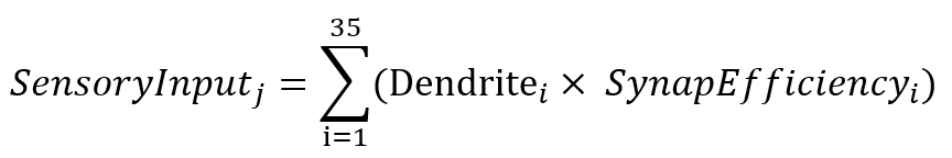
In this setup, neuron j receives input from all 35 sensory units, scaled by synaptic efficiency. When a sensory unit fires, its signal contributes to the summation at each connected neuron—including neuron j.
Visualizing Neural Summation
To complete the background for understanding the neural summation equation, we shift from symbolic expressions to structural views. These diagrams offer a non-equation perspective on how inputs converge at each neuron in the receiving layer.
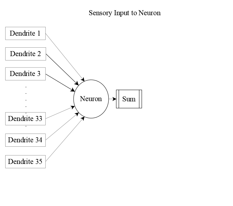
Each receiving neuron integrates signals from all 35 sensory units. These inputs arrive via dendrites and are scaled by synaptic efficiency.
But sensory input alone doesn’t tell the full story. Neurons in the receiving layer also send signals to one another, forming a web of lateral connections. Incorporating these interactions yields the complete input equation: neuron j receives 134 distinct inputs—35 from sensory units and 99 from its peers.
The structural view of these interconnections is shown below.
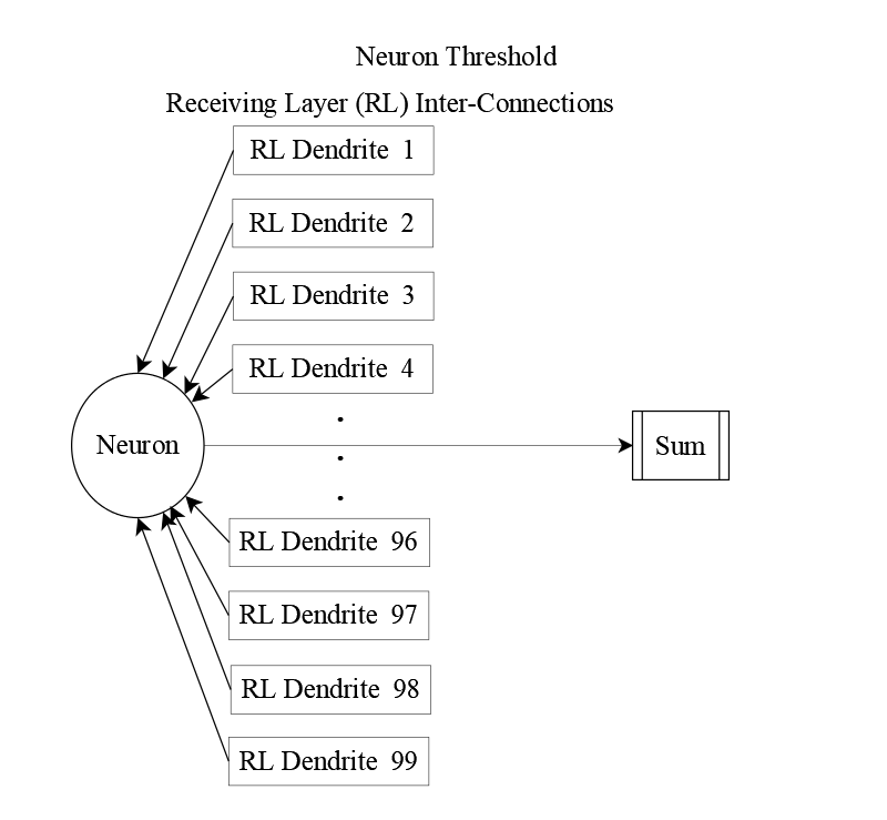
Bringing these perspectives together, we arrive at a full picture of how each receiving neuron sums its inputs—sensory and lateral—before comparing the result to its firing threshold.
Learning E: Recognition, Almost Gates, and Rejection
This neural network was trained on repeated presentations of English capital letters. Over several hundred exposures, the receiving layer stabilized—assigning specific neurons as “winning neurons” for each letter with over 95% consistency.
Neurochemical changes during development make certain ages especially primed for learning specific skills. These sensitive periods are explored further in Learning with Almost Gates, which discusses genetically timed sensitive and critical periods for learning.
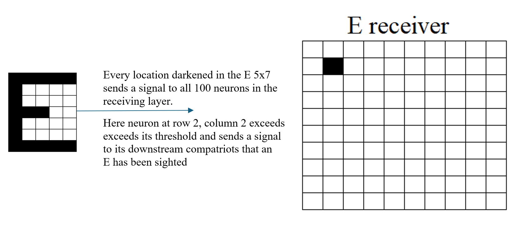
In this example, the network has learned to recognize the capital letter E. When the sensory pattern for E is presented, neuron (2,2) in the receiving layer exceeds its threshold and sends a signal to downstream neurons—indicating that an E has been sighted.
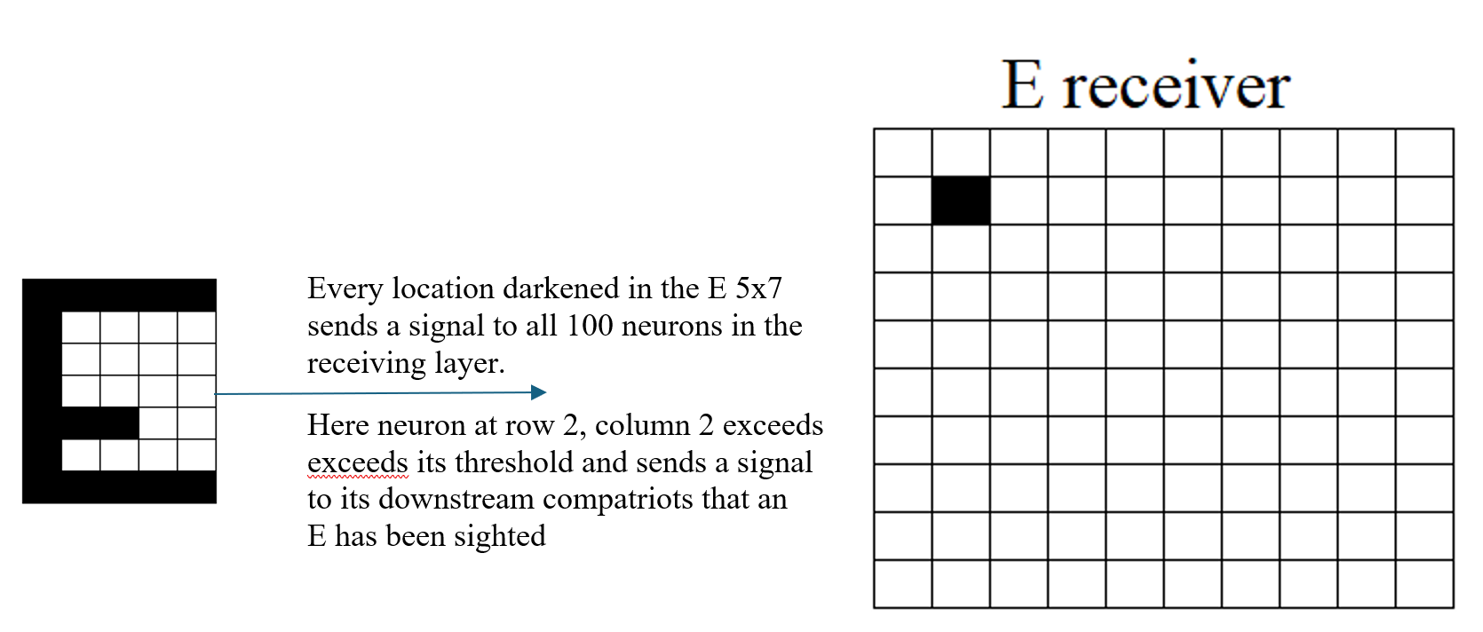
The Almost Gate mechanism allows the network to accept a slightly malformed version of E. Despite deviations from the canonical pattern, the input is close enough in structure—edges, intersections, and signal distribution—for the network to treat it as an E. Neuron (2,2) again fires, sending the same signal.
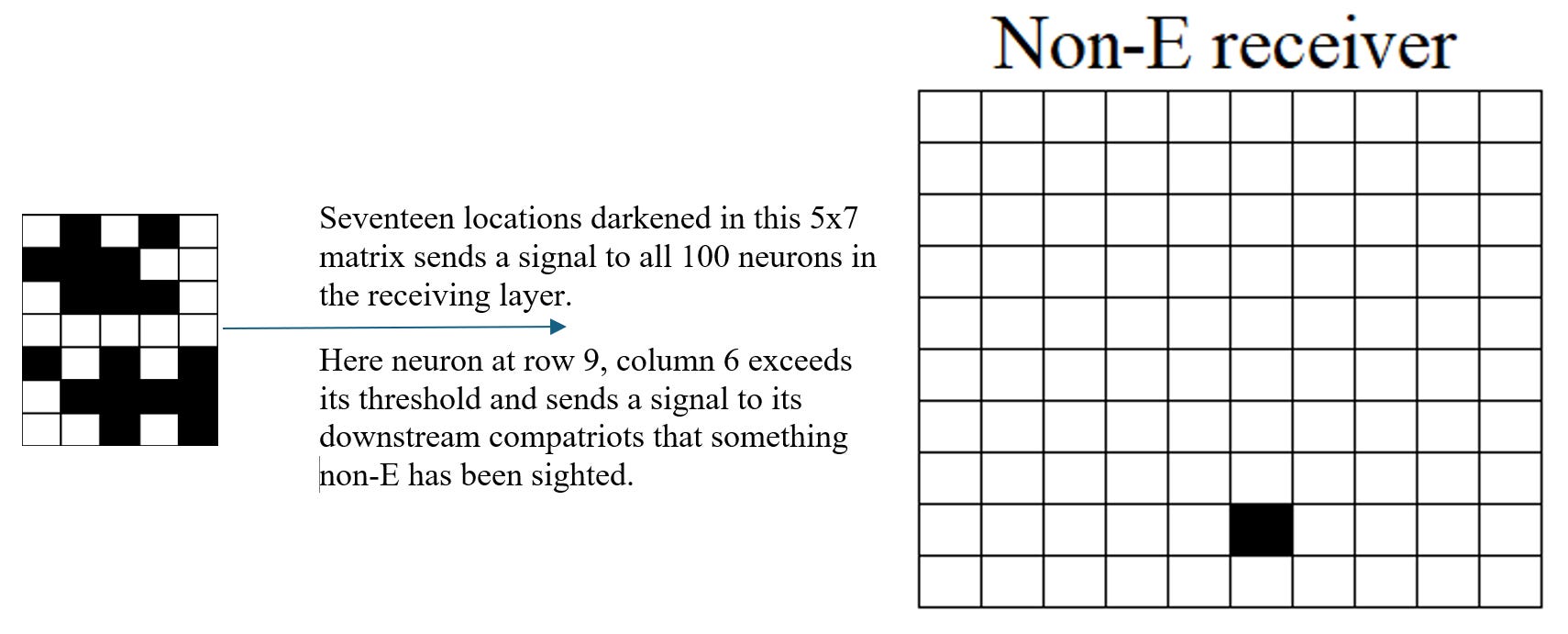
In contrast, a jumble of 17 active sensory cells fails to trigger recognition. Although the number of signals is the same, the spatial pattern lacks the structural features—such as aligned edges and intersections—that define E. The network does not categorize this input as E, and no signal is sent from neuron (2,2).
Abstraction Occurs in Both Hemispheres
Almost Gates abstract. They strip away anomalies when categorizing, allowing patterns to be recognized despite variation. Although illustrated here with sensory data, Almost Gates line the neural pathways through which memories and knowledge flow. As thought itself grows more abstract, the Cognitive Hierarchy Example shows the crucial role of Almost Gates in shaping higher-level reasoning.
These mechanisms operate across both hemispheres. In Cortical Columns and Our Thoughts, the left hemisphere’s pathways are traced as verbal descriptions pass through Almost Gates. On the right, Almost Gates work with patterns grounded in personal experience. Two Thoughts, One Brain: How We Decide follows these dual prefrontal pathways into their executive areas, where shared working memory integrates the two streams.
Genetic Variability
Almost Gates differ across people. Within an individual, their height is consistent, but genetic inheritance sets different thresholds from one person to another, and with it, the “height” of an individual’s Almost Gates.
High thresholds: Some people require near-perfect matches before categorizing. Their Almost Gates stand tall, demanding precision. This can foster meticulousness and caution—traits often seen in accountants, engineers, or others whose work prizes exactness.
Low thresholds: Others accept looser matches. Their Almost Gates sit lower, allowing broader associations and more fluid categorization. This can foster creativity and openness—traits often found in artists, designers, or improvisers.
These differences are not trivial. The height of one’s Almost Gates influences choices, perspectives, and even life paths. Where one person sees only noise, another sees possibility. Where one demands certainty, another embraces ambiguity. Genetic variability ensures that human cognition is not uniform, but richly diverse.
Almost Gate Surprising Start
Almost Gates begin shaping categories before language arrives. Even in infancy, they sort experience into patterns: who feeds you, the bodily warmth of satisfaction after eating, and the reliable comfort that follows a cry. These early categorizations lay the groundwork for self-image and confidence, as explored in 3S Imperatives to Emotions.
Abstract Substitution
When facing a stubborn problem or an abstract theory, progress often comes from substitution—replacing a narrow category with a broader one. Increased abstraction leads to more generalized matches that a tighter, more specific categorization would never have considered.
In the executive areas of the prefrontal lobes, working memory can then search for occasions when that broader category was active. Each retrieved memory carries details beyond the category itself—extra features that may unlock new approaches to the current dilemma.
Why does this matter? Because abstraction sometimes discards features or groups them in ways that prove unhelpful in novel situations. By deliberately stepping up to a more general category and re-examining memory, the mind can uncover overlooked angles. In difficult decisions, this capacity to reframe through substitution is often the key to fresh insight.
Individual Variability in Almost Gates
Earlier we noted that neural thresholds—and the height of the Almost Gate—are set by genetics. What follows is not uniform: each person’s gates stand at a different level.
Some demand many precise details before they will agree two items are similar. Others readily point out connections between disparate things, surprising friends who ask, “How can you say that?”
These differences shape perception, decision, and creativity.
Reflecting on your own Almost Gate may reveal why you notice certain patterns, resist others, and make choices in the way you do.
Almost Gate Linchpins
The Almost Gate is not a fanciful metaphor—it is grounded in the way neurons operate. A single neuron can receive an immense number of inputs, and many different combinations of signals can trigger its signal.
When a particular combination reappears, Hebb’s Law1 strengthens those connections, reinforcing the likelihood that the neuron will respond the same way in the future. At the same time, the All-or-None Principle2 ensures that once the threshold is crossed, the axon delivers a uniform signal—regardless of which exact inputs triggered the firing.
In practice, this means that all combinations exceeding the threshold are treated as identical after firing. That convergence of diverse inputs into a single, consistent output is the neural Almost Gate in action.
Citation
Mexican Hat Function. By JonMcLoone - Own work, CC BY-SA 3.0, https://commons.wikimedia.org/w/index.php?curid=18679602
Further Information
The Brain’s Gatekeeper. The Almost Gate in action.
Neurons: Engines of Signal Flow. Schematic of dendrites at synaptic gap of a neuron.
Layers of Neurons Yield Brain Maps. Implications of Almost Gates.
Learning with Almost Gates. Critical learning period and stages of learning.
3S Imperatives to Emotions. Why do we feel fear before we think?
Cortical Columns and Our Thoughts. Post with separate right and left paths identified.
Cognitive Hierarchy Example. How Meaning Emerges from Layered Abstraction.
Two Thoughts, One Brain: How Do We Decide. Neural pathways of the right and left hemispheres, functions, and resolution.
An important biological law was identified by Donald O. Hebb. Here it is defined in Scholarpedia.
“When an axon of cell A is near enough to excite B and repeatedly or persistently takes part in firing it, some growth process or metabolic change takes place in one or both cells such that A’s efficiency, as one of the cells firing B, is increased.
In The Portrait of the Brain, Adam Zeman (p 96–97) gives this evocative statement of the All-or-None principle.
[Neurons] accumulate a tiny electrical charge, with a higher concentration of negatively charged atoms and molecules inside the cell than outside it. This creates the opportunity for signaling. When the difference in charge between the inside and the outside of a neuron is reduced by a certain small amount, molecular gates in the cell membrane suddenly open, allowing a … wave of sodium influx travels down the output cable transmitting signals away from the cell … Here is the basis for the neuronal ‘action potential’, the all or nothing, binary signal that conveys the neuron’s crucial decision about whether or not to fire.